# Population,总体
# 总体均值设置为100
mu <- 100
# 总体标准差设置为15
sigma <- 15
# 随机种子值设置为2026
set.seed(202605)
# 将ID与IQ存入数据表中
population10000 <- data.frame(
  # 生成10000个ID(被试编号)
  ID = seq(1:10000),
  # 生成10000个均值为mu、标注差为delta的IQ分数
  IQ = round(rnorm(10000, mean = mu, sd = sigma), 0)
  )
# 查看数据表
# View(population10000)
# 查看数据表前6行
range(population10000$IQ)
## [1]  38 156
head(population10000)
##   ID  IQ
## 1  1 126
## 2  2  94
## 3  3  93
## 4  4 119
## 5  5 104
## 6  6  81
# 总体的实际均值
mean(population10000$IQ)
## [1] 99.8009
# 总体的实际标准差
sqrt(sum((population10000$IQ - mean(population10000$IQ))^2)/10000)
## [1] 14.94354总体分布,样本分布,抽样分布
Polulation, sample, and sampling distributions
1 总体
我们捏造一个人数为10000人的总体,为10000名被试设定编号ID,并捏造出其IQ数据,设定IQ的均值为100,标准差为15。
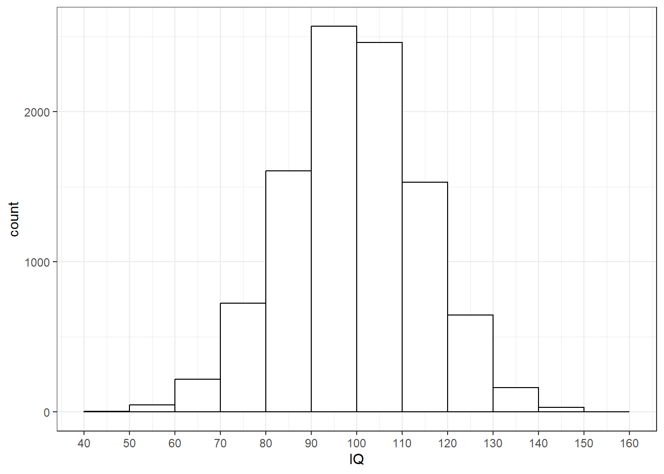
2 总体分布
总体分布(population distribution)是总体(10000名被试IQ得分)的分布。注意该分布的横纵坐标的全距。
3 取样过程
接下来,我们模拟取样的过程。我们从N = 10000的总体中随机抽取一个样本量n = 100的样本。我们称这个样本为sample1。
4 样本1
查看sample1中的数据。注意:被试ID的顺序是乱的,这是由随机取样导致的。
5 基于样本1估计总体均值与标准差
样本的均值是总体均值的无偏估计。样本的标准差总是小于总体的标准差,因此使用样本的无偏标准差作为总体标准差的无偏估计。尽管名为“无偏”,实际上还是有偏差的。
# 取值范围
range(sample1$IQ)
## [1] 67 139
# 计算sample1的IQ的均值
sample1_mean <- mean(sample1$IQ)
sample1_mean
## [1] 98.93
# 计算sample1的IQ的标准差
sample1_sd <- sqrt(sum((sample1$IQ - sample1_mean)^2)/100)
sample1_sd
## [1] 14.04511
# sample1的无偏标准差(基于sample1估计总体的标准差)
sample1_sd_unbiased <- sqrt(sum((sample1$IQ - sample1_mean)^2)/(100 - 1))
sample1_sd_unbiased
## [1] 14.11587
# 使用`sd()`函数计算sample1的无偏标准差(总体标准差的估计值)
sd(sample1$IQ)
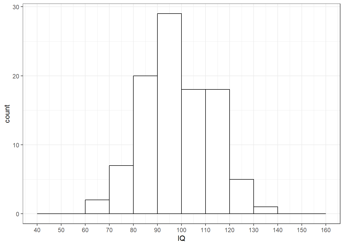
## [1] 14.115876 样本分布:样本1的分布
样本分布(sample distribution)是样本中100个被试IQ得分的分布。
7 样本分布与总体分布的关系
若总体的均值mu与标准差sigma是未知的,我们可以用样本的均值与无偏标准差来估计总计的均值与标准差:
\[\begin{align} mu &= M_{sample} \\ sigma &= s \end{align}\]
在上式中,\(M_{sample}\)是样本的均值,\(s\)是样本的无偏标准差。
8 重复取样
使用一个样本计算得到的均值估计总体的均值产生的偏差可能较大,如果我们重复取样的过程,抽取多个样本,将多个样本的均值求均值,那么,我们将得到更为准确的估计值。下面,我们从人数N = 10000的总体中取出m = 1000个样本量n = 100的样本。
# 从总数为10000的样本中累计抽取1000个样本量为100的样本,存入samples
samples <- list()
for (index in 1:1000) samples[[index]] <- population10000[sample.int(10000, 100), ]
# 查看samples
length(samples)
## [1] 1000
head(samples[[1]])
##        ID  IQ
## 989   989 107
## 194   194 115
## 3489 3489 104
## 4818 4818 144
## 7487 7487 122
## 3070 3070 117
9 抽样分布:1000个样本的均值的均值与标准差
与单个样本(例如:sample1)相比,1000个实际样本的均值的均值更加接近总体均值。
# 分别计算1000个样本的均值,一共得到1000个均值,存入samples_means
samples_means <- sapply(samples, function(x) mean(x$IQ))
head(samples_means)
## [1] 101.21 98.14 100.45 100.09 100.32 98.57
range(samples_means)
## [1] 95.35 104.40
head(samples_means)
## [1] 101.21 98.14 100.45 100.09 100.32 98.57
# 1000个实际样本的均值的均值。
mean(samples_means)
## [1] 99.8118
# 1000个实际样本的均值的方差。
sum((samples_means-mean(samples_means))^2)/1000
## [1] 2.023013
# 1000个实际样本的均值的标准差。
sqrt(sum((samples_means-mean(samples_means))^2)/1000)
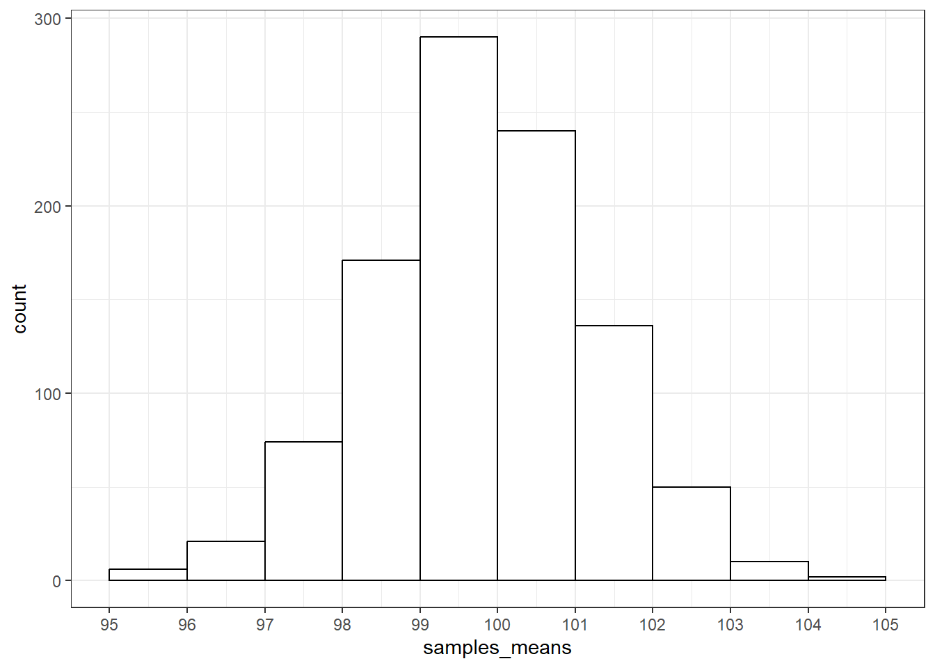
## [1] 1.42232710 抽样分布
抽样分布是1000个样本的均值的分布。这个分布中的每一个数据点是一个样本中100名被试的IQ的均值,而不是一个被试的IQ得分,这个分布的中心是是1000个样本的均值的均值,这个分布的标准差是1000个样本的均值的标准差。
11 抽样分布与总体分布、样本分布的关系
若总体的均值mu与标准差sigma是已知的:
\[\begin{align} M_{sampling} &= mu \\ SD_{sampling} &= \frac{sigma}{\sqrt{n}} \end{align}\]
在上式中,n是样本量。
若总体的均值mu与标准差sigma是未知的,我们可以用样本的均值与无偏标准差来估计总计的均值与标准差:
\[\begin{align} M_{sampling} &= M_{sample} \\ s_{sampling} &= \frac{s}{\sqrt{n}} \end{align}\]
在上式中,\(M_{sample}\)是样本的均值,\(s\)是样本的无偏标准差。
12 三种分布的比较
比较三种分布的频数分布图:
library(patchwork)
plot_pop <- ggplot(population10000, aes(x = IQ)) +
  geom_histogram(breaks = seq(40, 160, 10),
                 fill = "wheat",
                 color = "grey") +
  scale_x_continuous(breaks = seq(40, 160, 20)) +
  coord_cartesian(xlim = c(40, 160), ylim = c(0, 3000)) +
  labs(title = "Population") +
  annotate(geom = "text",
           label = c("N == 10000","mu == 99.80","sigma == 14.94"),
           x = 55, y = c(2300, 2000, 1700), parse = TRUE) +
  theme_classic()
plot_sample <- ggplot(sample1, aes(IQ)) +
  geom_histogram(breaks = seq(40, 160, 10),
                 fill = "wheat",
                 color = "grey") +
  scale_x_continuous(breaks = seq(40, 160, 20)) +
  coord_cartesian(xlim = c(40, 160), ylim = c(0, 30)) +
  labs(title = "Sample") +
  annotate(geom = "text",
           label = c("n == 100","M == 98.93","SD == 14.12"),
           x = 55, y = c(23, 20, 17), parse = TRUE) +
  theme_classic()
plot_sampling <- ggplot(data.frame(samples_means), aes(samples_means)) +
  geom_histogram(breaks = seq(95, 105, 1),
                 fill = "wheat",
                 color = "grey") +
  scale_x_continuous(breaks = seq(95, 105, 1)) +
  coord_cartesian(ylim = c(0, 300)) +
  labs(title = "Sampling", x = "Mean of IQ") +
  annotate(geom = "text",
           label = c("m == 1000","M[mean] == 99.81","SD[mean] == 1.42"),
           x = 96.3, y = c(230, 200, 170), parse = TRUE) +
  theme_classic()
plot_pop + plot_sample + plot_sampling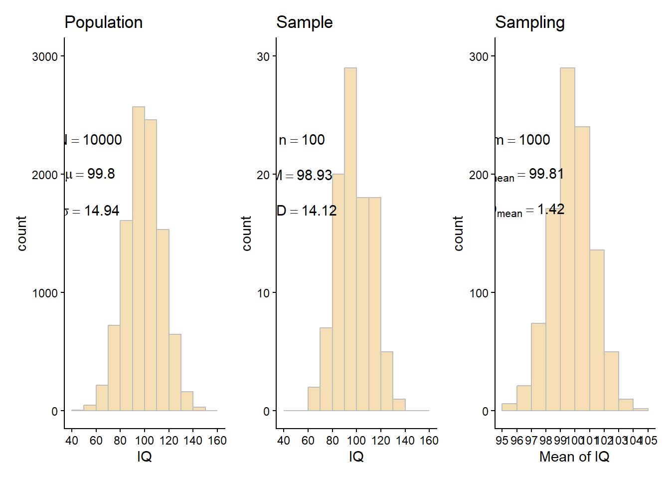
本文到此结束。